Here is a summary of my talk at the BLAST analysis meeting, http://
blast.lns.mit.edu/PRIVATE_RESULTS/USEFUL/ANALYSIS_MEETINGS/
meeting_060419/rad_blast-2006-04-19.ppt . Since it caused some
controversy, I am including extra details so anyone interested can
verify my arguments. I have tried to present it in a more coherent
manner, and I apologize in advance for the length of it, but please
read it in full before responding.
I. Mascarad Radiative Tail
A. Kinematics -- inelasticity v = W^2 - M^2, W^2 = M^2 + 2
M \nu - Q^2. The two other photon variables (tau, phi_k) are
integrated over.
B. Cutoffs -- In integrating the radiative tail, there are two
cutoffs in 'v' to consider:
1) Upper cutoff, used to match the experimental cuts.
2) Lower cutoff, used historically to avoid the infrared
divergence (copious soft photon emission). This cutoff is now
avoided in MASCARAD by proper renormalization, in which the infinite
vertex correction (I.C.2) at the pole cancels the divergent integral
of the tail at low v (I.C.3). However, because the infinities are in
different places, they only cancel in the integral over 'v'.
Therefore, in a Monte Carlo generator, the elastic pole must also
include the radiative tail up to some low cutoff 'v', which should be
less than the BLAST resolution.
C. Details -- MASCARAD calculates the cross section in
different parts:
1) the Born (tree level) amplitude.
2) virtual elastic -- contribution to the elastic cross
section (same kinematics) from vertex corrections and loop diagrams.
3) the soft radiative part -- basically the part same as used
in Mo & Tsai. This includes the infrared divergent part.
4) finite radiative correction -- the remaining contributions
to the exact calculation of the radiative tail. This part is a
function of \vec p_k, the photon 3-momentum. It is actually a small
negative correction to (3), and cannot be used alone. (see values in
attachment)
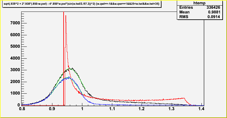
D. Cross section -- Mascarad outputs one final number: delta
(v) = (integral of radiative cross section from elastic peak up to
'v') / (Born cross section). The radiative invariant mass spectrum
including the tail equals: sigma_Born * d(delta)/d(v), (after
transforming to W). Discretely, delta(v0)=pole+soft photons<v0;
delta(v1)-delta(v0) = first bin of tail, etc. This is the blue fill
histogram in slide 2. The pole (100x greater than the first bin of
the tail) is omitted, but its area is equivalent to the yellow fill
histogram. I attached a data-file of delta(v) for 5 Q^2 bins. It
was generated by adding two parts: delta_soft(v) (I.C.1-3) calculated
on the same grid, and delta_hard(v) (I.C.4) calculated on a much
coarser grid to save computation time.
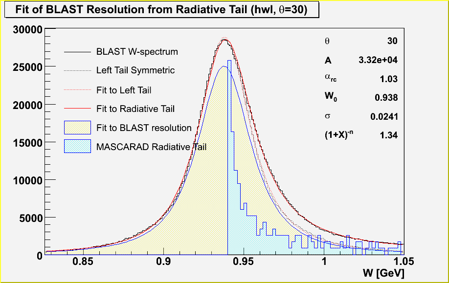
II. BLAST Invariant Mass Spectrum
A. Data -- shown as the black histogram, simply a plot of W
from the elastic data with the minimal cut of "qwl==-1 && qwr==1 &&
25 < twl && twl < 35" (left sector). I only go to 1050 MeV to avoid
inelastic contributions to the cross section (pion threshold ~ 1070
MeV).
B. Resolution (generalized) -- shown as the yellow fill curve;
don't worry for the moment how it was obtained. This is actually the
BLAST response function to a delta pole, \delta(W-M). For example,
this would be what we measured if there were no radiation. It has
been offset by M=.938 for visual effects, but is actually centered
very close to 0 MeV. The shift from zero (W_0-M) is just the
kinematic offsets we normally talk about, and the width is the BLAST
resolution. But these are just two characteristics of the BLAST
response; another might be the strength of the tail. The integral
must be less than unity (i.e. the conversion factor between yield and
cross section) and equals the BLAST efficiency.
C. Convolution -- shown as the red curve, the theoretical cross
section convoluted with the BLAST response should equal the measured
W-spectrum according to the definition of (B).
D. Assumptions -- there was very good agreement of the
convolution (red curve) with data (black histogram). However, there
were a number of assumptions made:
1) The response is independent of momentum (there's no way
around this; otherwise you can't de-convolute the W-spectrum).
2) I also assumed that it is symmetric in W. In theory there
is no problem with relaxing this constraint, although it would be
more difficult to extract the strength of the radiative tail, and one
would just have to blindly trust the MASCARAD calculation.
E. Computer Code -- this is all implemented in 'blast/exp/
analysis/macros/fit_invmass.C' In particular, there are two
functions defined:
1) 'res_fn' -- implements the BLAST response (II.B), but
shifted by 'M=.938'. See below for details of the free parameters.
2) 'rad_fn' -- calculates the convolution of 'res_fn' with
the radiative cross section (I.D).
III. Shift in Elastic Peak due to Radiative Tail
A. Result -- 0.8 MeV. This is just the difference in the peaks
of the blue curve (II.B) and the red curve (II.C). Or in other
words, the difference between the BLAST response to the elastic peak
(note f(x) convoluted with delta(x-x0) = f(x0)) and the BLAST
response to the radiative cross section. And actually for this
analysis, the shape of the response function is immaterial; the shift
of the elastic peak _ONLY_ depends on the width of the response
function you use (the BLAST resolution). In particular, clearly the
offset 'W_0' and amplitude 'A' have no effect on the shift, as seen
from the properties of convolution.
B. Resolution dependence -- the shift of the convolution was
repeated for three resolutions: 25,50,100 MeV (side 4), resulting in
shifts in W of about 1,2,4 MeV.
C. Caveats -- there are three things which I can think of which
may affect the results, none of which are the above methodology. I
would prefer to deal with these issues before trying different
response functions, as different people have suggested.
1) MASCARAD calculates radiative corrections for fixed Q^_l,
defined by Q^2_l = 4 E E' sin^2(\theta_e/2). I histogrammed the
invariant mass spectrum with a cut on \theta_e instead, which only
coincides with Q^2_l on the elastic ridge.
2) I binned the radiative tail starting at W=940MeV in steps
of 2MeV. You see that most of the contributions come from the first
bin, and it is very steep. So calculating the radiative tail with
finer bins can potentially have a big impact. I also note that DGen
starts it's tail at v=0.10 ~ dW=5.3 MeV, so it may also be affected
by the same issue.
3) In order to account for multiple photon emission, MASCARAD
exponentiates the integral of the soft part of (I.C.3). So if your
lower cutoff is too small, multiple photon emission will not be
properly accounted for. My analysis actually did not use a lower
cutoff (only DGen), but I'm not sure what effect this has on the
derivative d(delta)/dv.
D. Shift of Mean -- this can be much larger, but depends on the
exact details of cuts and fitting. However, note that the shift of
the mean with respect to the mode (peak) can be extracted from the
data themselves, and does not need to be simulated. The only
important thing is to remain consistent with your analysis.
< interlude: The above is fairly straight-forward and we already
have the radiative correction, but I went one step farther and
extracted the BLAST response function from the W-spectrum of the
data. This is the controversial part, explained below. >
IV. Extraction of the BLAST response function (resolution).
A. Approach -- the basic idea is to de-convolute the radiative
cross section from the BLAST resolution. The caveats in (II.C) and
(III.B) apply. Of course one could de-convolute by dividing the
Fourier transforms, but you would end up with an ugly function, and
I'm not sure how reliable this method is. I chose to parameterize
the response with a simple analytic function, and fit the convolution
with the radiative cross section for the free parameters, as
discussed below. The whole process is computed in the code
'fit_invmass.C'. I would like to emphasize that this step is just as
important for testing MASCARAD against our data as it is for actually
extracting the response function. It is the ONLY way to compare our
data against MASCARAD.
B. Left Tail Symmetric -- (black dotted histogram) I mention it
in passing because it was used to determine general features of the
response function. The idea is that radiation is mostly on the right
side of the peak. However, this is NOT the BLAST resolution, since
the radiation also bleeds in from smearing out the tail; just compare
it with the yellow fill curve to see how much!
C. Response Function -- ('res_fn') I chose the
parametrization '[A]/(1+(W-[W_0])/[sigma]))^[n]'. I tried a
Gaussian, but it had the wrong shape in the tails (as expected). A
pure Lorentzian had good tails, but could not reproduce the peak.
Adding combinations of the two or multiplying by '(1-k*gaus)'
produced funny-looking functions with extra wiggles. So this is
purely phenomenological, but matches the data real good, ant least
for small theta. At higher theta, the momentum resolution is a mess,
even double-valued, so not much you can do there. No constant offset
was needed, as there is essentially no background.
D. Convolution Function -- ('rad_fn') This is just a numerical
convolution of 'res_fn' with the elastic pole and each bin of the
radiative tail (blue). However, I added one extra parameter,
[alpha_rc], a scale factor for the radiative tail only (not the
elastic peak). The purpose of this parameter was to test the
validity of MASCARAD. A fit of close to '1' indicates that MASCARAD
calculates the proper strength of the tail or, turning the argument
around, that the fit was done properly. For final results, one
should really fix 'alpha_rc' to 1.
E. Results -- the red curve (IV.D). The parameters of this
curve are shown at the right, but most of these parameters were
directly passed to the resolution function, the yellow fill curve
(IV.C). This is the unique function, which can be convoluted with
the radiative cross section to match up with the BLAST yield, and is
NOT a circular argument.
< the end. now miscellaneous issues: >
V. Investigation of MC Reconstruction
A. Source -- I used Adrian's MC file generated with DGen +
Mascarad. See his email in BLAST_TALK, 2006-04-13.
B. 'lrn' bug -- The problems I reported to BLAST_TALK,
2006-04-17 were caused by 'lrn' booking a photon instead of the
electron or proton. I fixed it to preferentially book charged
particles, and checked it in.
C. MC reconstruction -- after this fix, I was able to compare
the generated (thrown) kinematical variables (red, top left figure,
slide 5) with the reconstructed ones: with a cut on the elastic part
(blue), or all events (black). The elastic pole was peaked at W=948
MeV, and the complete reconstructed spectrum at W=958 MeV. This is
dramatically greater than the shift reported above. I did check my
calculation for an obvious error and found none. Part of it is
definitely due to reconstruction (ie. the blue curve should have no
shift), but another explanation may be the magnitude of the tail
(VI.B). Repeating (III.A) with a 3.3x larger tail, I get a shift of
the peak of 2.3 MeV instead of 0.9 MeV.
D. Log file -- attached as 'mc_gen_recon.log'
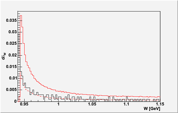
VI. Comparison of original MASCARAD with translation into DGen.
A. Test -- I compared the generated radiative tail (V.A, red)
with the radiative tail calculated by the original MASCARAD (I.D,
black), shown in the lower left (left sector, \theta_e=30 deg), and
right (left,right sector; \theta_e=30,40,50,60,70 deg) panels of
slide 5. The plots are in units of d(delta)/dv. The black curve was
already normalized; the the red was scaled by normalizing the pole
(v<0.010) to the value 'delta(0.010)', calculated from the original
Fortran code. The dotted red histogram has been scaled to best match
the black curve. This scale factor is reported in the results.
B. Results -- the DGen code generates a radiative tail 2.4--3.3
times larger than expected. The left and right sectors were consistent.
C. Log file -- attached as 'dgen_masc.log'
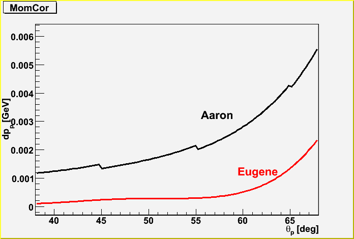
VII. Comparison of ELOSS calculations.
A. Aaron's calculation -- see BLAST_TALK, 2004-12-03
B. Eugene's calculation -- see plot in BLAST_TALK, 2006-02-22
12:52, or parametrization
C. Computer code -- 'eloss_aaron_eugene.C' compares
parametrizations
D. Results -- slides 6 and 7: Aaron's plot agrees with
Eugene's, but the parametrizations look off by a factor of 2.
I will continue to pursue radiative corrections, energy loss, and
report on the final geometric offsets after someone (not me!) has
resolved these issues.
--Chris
_______________________________________
TA-53/MPF-1/D111 P-23 MS H803
LANL, Los Alamos, NM 87545
505-665-9804(o) 665-4121(f) 662-0639(h)
_______________________________________
This archive was generated by hypermail 2.1.2 : Mon Feb 24 2014 - 14:07:33 EST